Collinearity and ridge regression

In statistics, collinearity (also multicollinearity) is a phenomenon in which one feature/predictor variable in a regression model is highly correlated with another feature variable.

In mathematics, a set of vectors $v_1,v_2,\ldots,v_n$ (e.g. a set of column vectors of predictors) are linearly dependent if there are constants $a_1,a_2,\ldots,a_n$, not all zero, such that $$a_1v_1+a_2v_2+ \cdots + a_nv_n = 0$$

In other words some combination of predictor columns (vectors), after scaling and adding them together, equal one or more other predictors.

If the predictors are linearly dependent, they are correlated, and this means the regression coefficients are not uniquely determined.

Example:

In this example we will simulate what happens with linearly dependent predictors.

Base example: ordinary regression

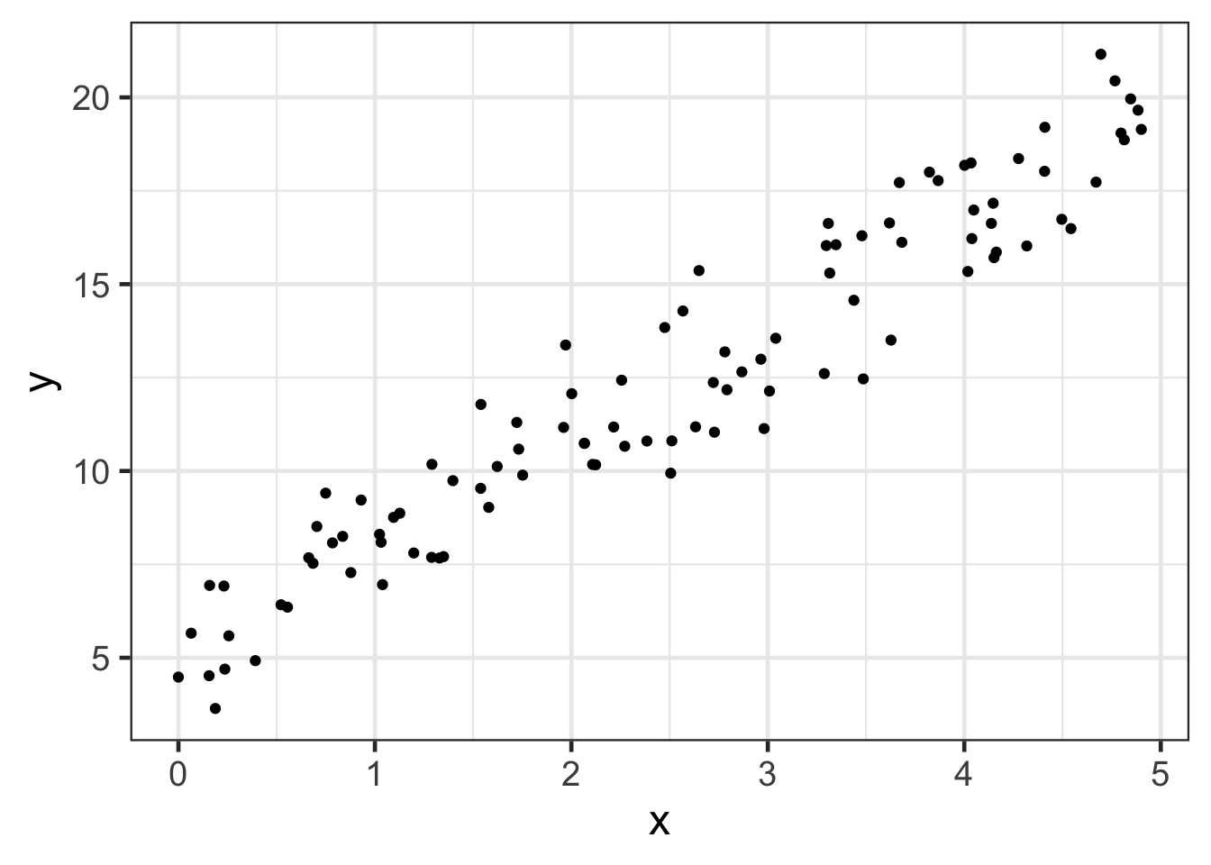
First we’ll create a simple dataset with one outcome and one predictor and estimate the coefficients with repeated regressions. In the dataset described by $5 + 3x$, i.e. intercept 5 and slope 3. There is no linear dependence as we have only one predictor.

> set.seed(8740)
> 
> # N rows
> N <- 100
> # predictor x runs from 0-5 in steps of 5/N plus a bit of noise
> x <- seq( 0, 5, 5/(N-1) ) + rnorm(N, 0, 0.1)
> 
> # when we regress y on x we should: 
> #   - estimate an intercept close to 5 
> #   - estimate the coefficient of x as close to 3 
> dat0 <- 
+   tibble::tibble( 
+     x = x 
+     # y is linearly related to x, plus some noise
+     , y = 5 + 3*x + rnorm(N, 0, 1.5)
+   )
> 
> dat0 %>% 
+   ggplot(aes(x = x, y = y)) +
+   geom_point()
> lm(y~x, dat0)

Call:
lm(formula = y ~ x, data = dat0)

Coefficients:
(Intercept)            x  
      5.100        2.895  

We see that an ordinary linear regression gives us results that are close to what we expect.

Now we do the same regression on similar data (only the noise is different) and take the mean values of the coefficient estimates:

> # create a list with 100 elements,
> # just so we run the regression 100 times
> 1:100 %>% as.list() %>% 
+   # for each element of the list, run the function 
+   purrr::map(
+     .f = function(...){ # we don't use any of arguments
+       # run the regression on the same data
+       tibble::tibble( 
+         x = x 
+         # y is linearly related to x, plus some noise
+         , y = 5 + 3*x + rnorm(N, 0, 1.5)
+       ) %>% lm(y~., .) %>% 
+         # extract the intercept and coefficient
+         broom::tidy() %>% 
+         dplyr::select(1:2) 
+     }
+   ) %>% 
+   # combine all the estimates
+   dplyr::bind_rows() %>% 
+   dplyr::group_by(term) %>% 
+   # summarize the combined estimates
+   dplyr::summarize(
+     mean = mean(estimate)
+     , variance = var(estimate) 
+   ) 

# A tibble: 2 × 3
  term         mean variance
  <chr>       <dbl>    <dbl>
1 (Intercept)  4.98  0.0705 
2 x            3.00  0.00732

We see that we are means of the coefficient estimates are close to what we expect.

Base example: ordinary regression with colinearity

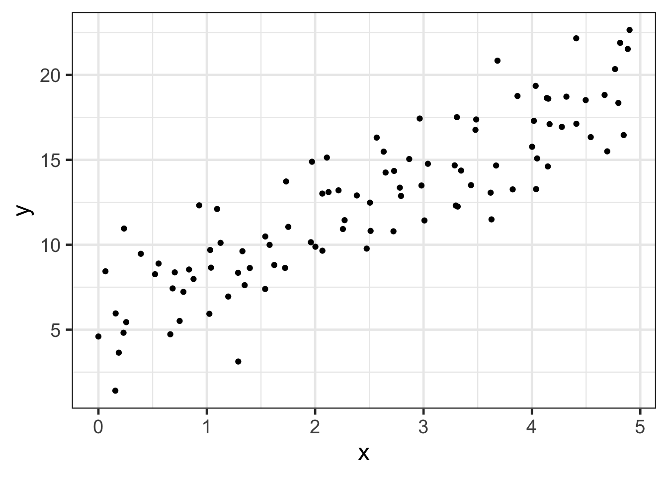
Now we create two colinear predictors $a,b$ as in the code below, where $b=2\times a$ so $a,b$ are collinear, $a+b=x$ , and the regression estimates two coefficients $\beta_a,\beta_b$ such that

$$\beta_a\times a+ \beta_b\times b = \frac{\beta_a}{3}\times x + \frac{2\beta_b}{3}\times x \rightarrow \frac{\beta_a}{3} + \frac{2\beta_b}{3} = 3$$

> dat1 <- 
+   tibble::tibble( 
+     a = x/3 + rnorm(N,0, 0.01)
+     , b = x*2/3 + rnorm(N,0, 0.01)
+     , y = 5 + 3*(a+b) + rnorm(N, 0, 2)
+   )
> 
> dat1 %>% 
+   ggplot(aes(x = x, y = y)) +
+   geom_point()
> lm(y ~ a + b, dat1)

Call:
lm(formula = y ~ a + b, data = dat1)

Coefficients:
(Intercept)            a            b  
      5.450       26.721       -9.104  

Sure enough, we have $\frac{\beta_a}{3} + \frac{2\beta_b}{3} \approx 3$. The code below performs the check:

> lm(y ~ a + b, dat1) %>% broom::tidy() %>% dplyr::select(1,2) %>% 
+   tidyr::pivot_wider(names_from = term, values_from = estimate) %>% 
+   dplyr::mutate(
+     check = a/3 + 2 * b/3
+   )

# A tibble: 1 × 4
  `(Intercept)`     a     b check
          <dbl> <dbl> <dbl> <dbl>
1          5.45  26.7 -9.10  2.84

Note that we have two unknowns, but only one equation, so the problem does not have a unique solution, as seen by the wide variation of estimates in a repeated regression:

> # create a list with 100 elements,
> # just so we run the regression 100 times
> 1:100 %>% as.list() %>% 
+   # run the 
+   purrr::map(
+     .f = function(...){ # we don't use any of arguments
+       # run the regression on the same data
+       tibble::tibble( 
+         a = x/3 + rnorm(N,0, 0.01)
+         , b = x*2/3 + rnorm(N,0, 0.01)
+         , y = 5 + 3*(a+b) + rnorm(N, 0, 2)
+       ) %>% lm(y~., .) %>% 
+         # extract the intercept and coefficient
+         broom::tidy() %>% 
+         dplyr::select(1:2) 
+     }
+   ) %>% 
+   # combine all the estimates
+   dplyr::bind_rows() %>% 
+   dplyr::group_by(term) %>% 
+   # summarize the combined estimates
+   dplyr::summarize(
+     mean = mean(estimate)
+     , variance = var(estimate) 
+   ) 

# A tibble: 3 × 3
  term         mean variance
  <chr>       <dbl>    <dbl>
1 (Intercept)  4.99    0.176
2 a            2.99  304.   
3 b            3.01   76.2  

Granted this is an extreme case of collinearity, but it illustrates the issue.

How can we mitigate the problem?

Ridge regression example:

Indeterminancy of the predictor coefficient estimates is a symptom of collinearity, as indicated by the large variance of the estimates.

Ridge regression penalizes large predictor coefficients, and we can use it here to address the collinearity.

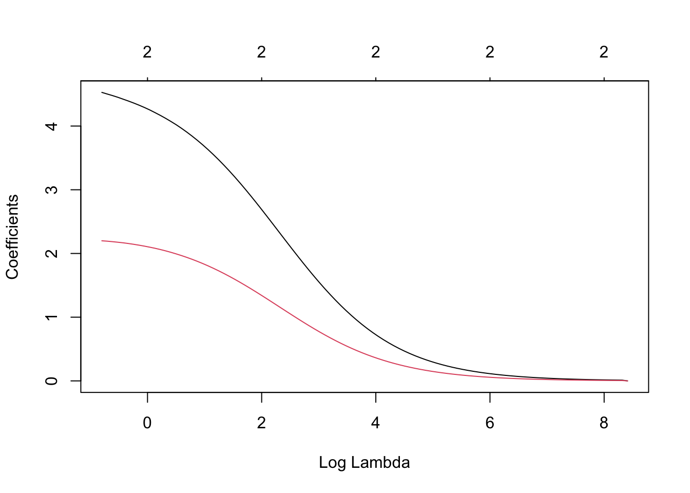
For the similar data (same relation between y and x, but different noise) under ridge regression (glmnet::glmnet with alpha=0):

> # create the dataset
> dat1 <- 
+   tibble::tibble( 
+     a = x/3 + rnorm(N,0, 0.01)
+     , b = x*2/3 + rnorm(N,0, 0.01)
+     , y = 5 + 3*(a+b) + rnorm(N, 0, 2)
+   )
> 
> # fit with glmnet (no cross validation and a range of penalty parameters)
> fit1 = glmnet::glmnet(
+   y = dat1$y
+   , x = model.matrix(y ~ a + b, data = dat1)
+   , alpha = 0
+ )
> 
> # plot the coefficient estimates as a function of the penalty parameter lambda
> plot(fit1, xvar='lambda')

Even using the defaults we can see that the coefficients estimated under the $l_2$ (sum of squared coefficients) penalty are in the right ballpark. The only step remaining is to find the best penalty coefficient $\lambda$.

We can do this with the built-in cross validation of cv.glmnet:: and alpha = 0, as follows:

> # fit with cv.glmnet (cross validation and a range of penalty parameters)
> fit_cv <- glmnet::cv.glmnet(
+   y = dat1$y
+   , x = model.matrix(y ~ a + b, data = dat1)
+   , alpha = 0
+ )
> 
> # get coefficients from fit1 with the penalty 
> # generating the smallest mse
> coef(fit1, s = fit_cv$lambda.min)
> # do the check
> fit1 %>% broom::tidy() %>% 
+   dplyr::filter(lambda == fit_cv$lambda.min) %>% 
+   dplyr::select(c(1,3)) %>% 
+   tidyr::pivot_wider(names_from = term, values_from = estimate) %>% 
+   dplyr::mutate(
+     check = a/3 + 2 * b/3
+   )

4 x 1 sparse Matrix of class "dgCMatrix"
                  s1
(Intercept) 5.405189
(Intercept) .       
a           4.528323
b           2.198966

# A tibble: 1 × 4
  `(Intercept)`     a     b check
          <dbl> <dbl> <dbl> <dbl>
1          5.41  4.53  2.20  2.98

So we can see that penalized regression, and in particular ridge regression, is useful for mitigating collinearity.