# Load libraries, get data & set seed for reproducibility ---------------------
set.seed(123) # seef for reproducibility
library(glmnet) # for ridge regression
library(dplyr) # for data cleaning
library(psych) # for function tr() to compute trace of a matrix
data("mtcars")
# Center y, X will be standardized in the modelling function
y <- mtcars %>% select(mpg) %>% scale(center = TRUE, scale = FALSE) %>% as.matrix()
X <- mtcars %>% select(-mpg) %>% as.matrix()
# Perform 10-fold cross-validation to select lambda ---------------------------
lambdas_to_try <- 10^seq(-3, 5, length.out = 100)
# Setting alpha = 0 implements ridge regression
ridge_cv <- cv.glmnet(X, y, alpha = 0, lambda = lambdas_to_try,
standardize = TRUE, nfolds = 10)
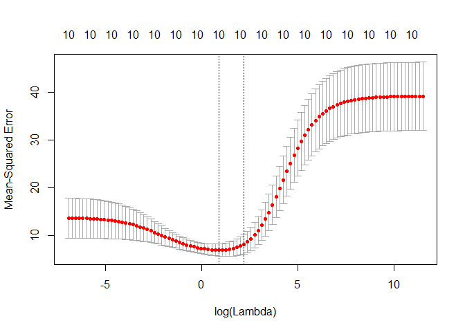
# Plot cross-validation results
plot(ridge_cv)Bias - Variance Trade-offs
Note
The following supplemental notes are based on this page. They are provided for students who want to dive deeper into the mathematics behind regularized regression. Additional supplemental notes will be added throughout the semester.
In the simple linear regression model, you have observations of the response variable with a linear combination of predictor variables where
where are all the parameters of the model. The vector of parameters are the weights or regression coefficients. Each coefficient specifies the change in the output that we expect if the corresponding input feature changes by one unit. The term is the offset or bias term, and specifies the output if all the inputs are zero. This captures the unconditional response, and acts as a baseline. We sometimes write the input as so the offset can be absorbed into the weight vector.
We can always apply a transformation (linear or non-linear) to the input vector, replacing with . As long as the parameters of the feature extractor are fixed, the model remain linear in the parameters even if not linear in the inputs.
Least squares estimation
To fit the linear regression model to data, we minimize the negative log-likelihood on the training set.
where the predicted response is . Focusing on just the weights, the NLL is (up to a constant):
We must estimate the parameter values from the data, and using the OLS method, the loss function is
which is minimized with the estimate
Bias and variance
The bias is the difference between the true population parameter and the expected estimator:
The variance uncertainty, in these estimates:
where is estimated form the residuals
This picture illustrates what bias and variance are.
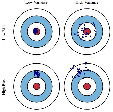
Both the bias and the variance are desired to be low, and the model’s error can be decomposed into three parts: error resulting from a large variance, error resulting from significant bias, and the remainder - the unexplainable part.
The OLS estimator has the desired property of being unbiased. However, it can have a huge variance. Specifically, this happens when:
- The predictor variables are highly correlated with each other;
- There are many predictors. This is reflected in the formula for variance given above: if m approaches n, the variance approaches infinity.
The general solution to this is: reduce variance at the cost of introducing some bias. This approach is called regularization and is almost always beneficial for the predictive performance of the model. To make it sink in, let’s take a look at the following plot.
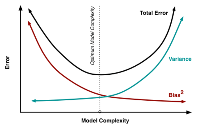
As the model complexity, which in the case of linear regression can be thought of as the number of predictors, increases, estimates’ variance also increases, but the bias decreases. The unbiased OLS would place us on the right-hand side of the picture, which is far from optimal. That’s why we regularize: to lower the variance at the cost of some bias, thus moving left on the plot, towards the optimum.
Ridge Regression
From the discussion so far we have concluded that we would like to decrease the model complexity, that is the number of predictors. We could use the forward or backward selection for this, but that way we would not be able to tell anything about the removed variables’ effect on the response. Removing predictors from the model can be seen as settings their coefficients to zero. Instead of forcing them to be exactly zero, let’s penalize them if they are too far from zero, thus enforcing them to be small in a continuous way. This way, we decrease model complexity while keeping all variables in the model. This, basically, is what Ridge Regression does.
Model Specification
In Ridge Regression, the OLS loss function is augmented in such a way that we not only minimize the sum of squared residuals but also penalize the size of parameter estimates, in order to shrink them towards zero:
Solving this for gives the the ridge regression estimates , where I denotes the identity matrix.
The parameter is the regularization penalty. We will talk about how to choose it in the next sections of this tutorial, but for now notice that:
- As ;
- As .
So, setting to 0 is the same as using the OLS, while the larger its value, the stronger is the coefficients’ size penalized.
Bias-Variance Trade-Off in Ridge Regression
From there you can see that as becomes larger, the variance decreases, and the bias increases. This poses the question: how much bias are we willing to accept in order to decrease the variance? Or: what is the optimal value for ?
There are two ways we could tackle this issue. A more traditional approach would be to choose λ such that some information criterion, e.g., AIC or BIC, is the smallest. A more machine learning-like approach is to perform cross-validation and select the value of λ that minimizes the cross-validated sum of squared residuals (or some other measure). The former approach emphasizes the model’s fit to the data, while the latter is more focused on its predictive performance. Let’s discuss both.
Minimizing Information Criteria
This approach boils down to estimating the model with many different values for and choosing the one that minimizes the Akaike or Bayesian Information Criterion:
where is the number of degrees of freedom. Watch out here! The number of degrees of freedom in ridge regression is different than in the regular OLS! This is often overlooked which leads to incorrect inference. In both OLS and ridge regression, degrees of freedom are equal to the trace of the so-called hat matrix, which is a matrix that maps the vector of response values to the vector of fitted values as follows: .
In OLS, we find that , which gives , where is the number of predictor variables. In ridge regression, however, the formula for the hat matrix should include the regularization penalty: , which gives , which is no longer equal to . Some ridge regression software produce information criteria based on the OLS formula. To be sure you are doing things right, it is safer to compute them manually, which is what we will do later in this tutorial.
Ridge Regression: R example
In R, the glmnet package contains all you need to implement ridge regression. We will use the infamous mtcars dataset as an illustration, where the task is to predict miles per gallon based on car’s other characteristics. One more thing: ridge regression assumes the predictors are standardized and the response is centered! You will see why this assumption is needed in a moment. For now, we will just standardize before modeling.