Principal Component Analysis (PCA) and Component Selection

PCA (short version)

Note

The PCA material here is taken from Probabilistic View of Principal Component Analysis

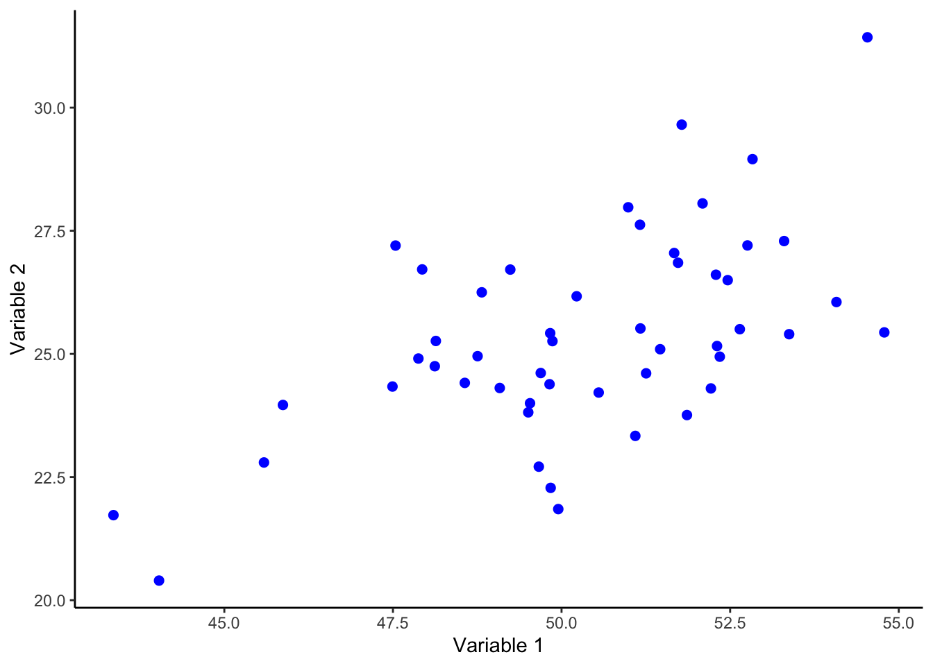
We’ll assume all columns in our data have been normalized - with zero mean and unit standard deviation.

Eigenvalue decomposition

For any square matrix $A$, $x$ is an eigenvector of $A$ and $\lambda$ the corresponding eigenvalue of $A$ if $Ax=\lambda x$. Suppose $A$ has a full set of $N$ independent eigenvectors (most matrices do, but not all).

If we put the eigenvectors into a matrix $Q$ (the eigenvectors are the column vectors of the matrix), then $AQ=Q\Lambda$, where $\Lambda$ is a diagonal matrix, with the eigenvalues on the diagonal. Thus

$$A = Q\Lambda Q^{-1} = Q\Lambda Q^\top \qquad(1)$$

This is the Eigenvalue Decomposition: a square $N\times N$ matrix ($A$) which is diagonalizable can be factorized as:

$$A = Q\Lambda Q^\top$$

where $Q$ is the square $N\times N$ matrix whose $i$th column is the eigenvector $q_i$ of $B$, and $\Lambda$ is the diagonal matrix whose diagonal elements are the corresponding eigenvalues. $Q$ is square and orthogonal ($Q=Q^{-1}=Q^\top$), because the eigenvectors are orthogonal.

SVD (Singular Value Decomposition)

If $A$ is not square we need a different decomposition. Suppose $A$ is an $N\times D$ matrix ($N$ rows and $D$ columns) - then we need a square, orthogonal $N\times N$ matrix $V$ to multiply on the right, and a square, orthogonal $D\times D$ matrix $U$ to multiply on the left. In which case our matrix (say A) can be factorized as:

$$A = U\Sigma V^\top \qquad(2)$$

$\Sigma$ will then be an $N\times D$ matrix where the $D\times D$ subset will be diagonal with $r$ singular values $\sigma_i\;i\in\{1,2,\ldots,r\}$ and the remaining entries will be zero.

We have

$$A = U\Sigma V^\top =\sigma_1u_1v_1^\top + \sigma_2u_2v_2^\top + \ldots+\sigma_ru_rv_r^\top$$ Note that this is a sum of matrices. The first is the best rank 1 approximation to $A$; the first $k$ is the best rank $k$ approximation to $A$

PCA decomposition

The PCA decomposition requires that one compute the eigenvalues and eigenvectors of the covariance matrix of $A$ (again an $N\times D$ matrix), which is the product $\frac{1}{n-1}AA^\top$. Since the covariance matrix is symmetric, the matrix is diagonalizable, and the eigenvectors can be normalized such that they are orthonormal.

The square corvariance matrix ($\frac{1}{n-1}AA^\top$) is symmetric and thus diagonizable, and so from equation (Equation 1), it can be factorized as:

$$\frac{1}{n-1}AA^\top = Q\Lambda Q^\top$$ where $\Lambda$ is the diagonal matrix with the eigenvalues of the covariance matrix and $Q$ has column vectors that are the eigenvectors of the covariance matrix.

However, using the SVD (Equation 2) we can also write

$$\frac{1}{n-1}AA^\top = \frac{1}{n-1} \left(U\Sigma V^\top\right)\left(V\Sigma U^\top\right) = U\Sigma^2U^\top$$

Using the SVD to perform PCA makes much better sense numerically than forming the covariance matrix to begin with, since the formation of $AA^\top$ can cause loss of precision.

Here is a simple PCA example:

Data

set.seed(1) # For data reproducibility
# create some data
dat1 <- tibble::tibble(
  x = rnorm(50, 50, sd = 3)
  , y = .5*x + rnorm(50, sd = sqrt(3))
)
# plot it
dat1 |> 
  ggplot(aes(x = x, y = y)) +
  geom_point(,color = "blue", size = 2) +
  xlab("Variable 1") +
  ylab("Variable 2") +
  theme_classic()

# center and
dat1 <- dat1 |>  
  dplyr::mutate(x = x - mean(x), y = y - mean(y))
# convert to matrix
dat2 <- dat1 |> dplyr::select(x,y) |> as.matrix()

Correlation

# Calculate the covariance matrix
cov_m <- (t(dat2) %*% dat2) / (nrow(dat2) - 1) 
cov_m

         x        y
x 6.220943 2.946877
y 2.946877 4.207523

# we can also use the cov function in base R
cov(dat2)

         x        y
x 6.220943 2.946877
y 2.946877 4.207523

PCA

# Use eigen() to obtain eigenvectors and eigenvalues
cov_e <- eigen(cov_m)

# Eigenvectors
e_vec <- cov_e$vectors

# Eigenvalues
e_val <- cov_e$values

# First eigenvector 
ev_1 <- e_vec[,1]

# Second eigenvector 
ev_2 <- e_vec[,2]

# eigenvectors are orthogonal and eigenvalues capture total variance
c( ev_1 %*% ev_2, e_val, e_val |> sum(), cov_m |> diag() |> sum())

[1] 2.749766e-17 8.328321e+00 2.100145e+00 1.042847e+01 1.042847e+01

For a positive semi-definite matrix SVD and eigendecomposition are equivalent. PCA boils down to the eigendecomposition of the covariance matrix. Finding the maximum eigenvalue(s) and corresponding eigenvector(s) can be thought of as finding the direction of maximum variance.

If we have a lot of data (many rows or many columns or both), we’ll have a large covariance matrix and large number of eigenvalues and their corresponding eigenvectors (though there can be duplicates).

Do we need them all? How many are just due to noise or measurement error? First look at random matrices, then at covariance matrices formed from random matrices.

Random Matrices

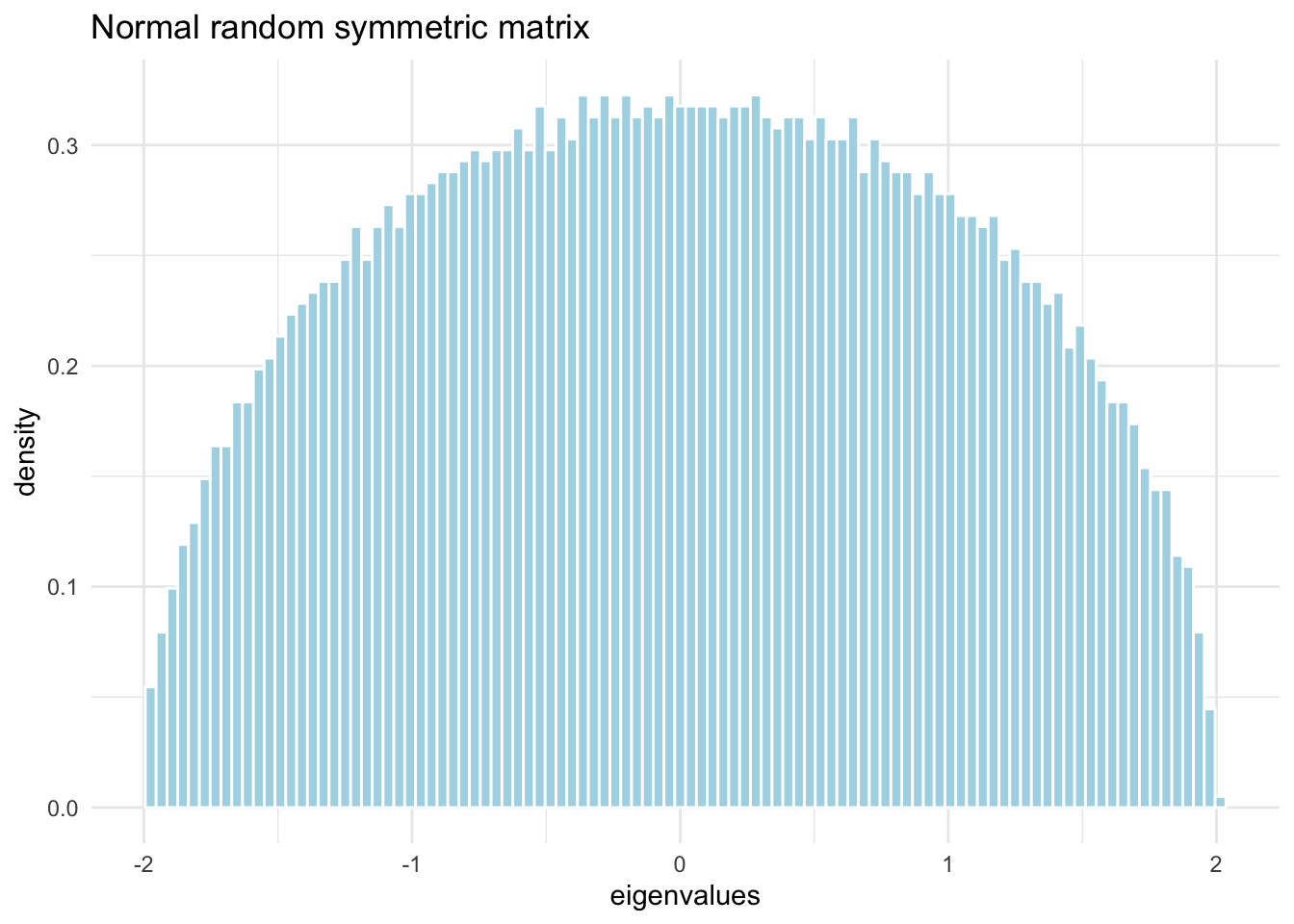
Let’s perform an experiment, generating a large random $N\times N$ data set using $N(0,1)$ measurements.

require(ggplot2, quietly=TRUE)

# 5000 rows and columns
n <- 5000
# generate n^2 samples from N(0,1)
m <- array( rnorm(n^2) ,c(n,n))
# make it symmetric
m2 <- (m + t(m))/sqrt(2*n) # t(m) %*% m
# compute eigenvalues and vectors
lambda <- eigen(m2, symmetric=T, only.values = T)

# plot the eignevalues
tibble::tibble(lambda = lambda$values) |> 
  ggplot(aes(x = lambda, y = after_stat(density))) + 
  geom_histogram(color = "white", fill="lightblue", bins=100) + 
  labs(x = 'eigenvalues', title = 'Normal random symmetric matrix') +
  theme_minimal()

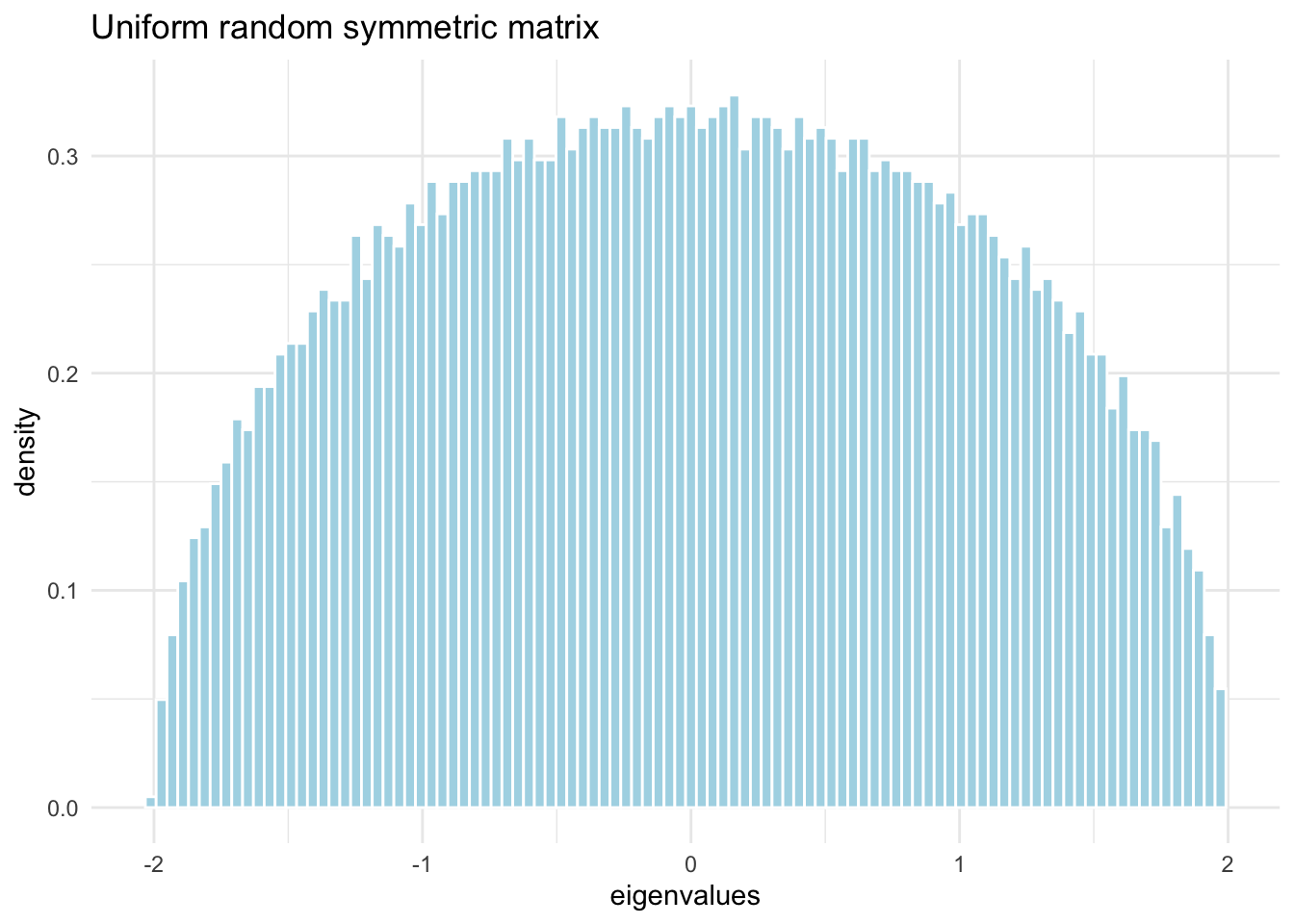
Let’s do the same, but with uniform $U(0,1)$ distributed measurements.

# 5000 rows and columns
n <- 5000
# generate n^2 samples from U(0,1)
m <- array( runif(n^2) ,c(n,n))
# make it symmetric
m2 <- sqrt(12)*(m + t(m) -1)/sqrt(2*n) # t(m) %*% m
# compute eigenvalues and vectors
lambda <- eigen(m2, symmetric=T, only.values = T)

# plot the eignevalues
tibble::tibble(lambda = lambda$values) |> 
  ggplot(aes(x = lambda, y = after_stat(density))) + 
  geom_histogram(color = "white", fill="lightblue", bins=100) + 
  labs(x = 'eigenvalues', title = 'Uniform random symmetric matrix') +
  theme_minimal()

Note the striking pattern: the density of eigenvalues is a semicircle.

Wigner’s semicircle law

Let $\tilde{A}$ be an $N\times N$ matrix with entries $\tilde{A}_{i,j}\sim\mathcal{N}\left(0,\sigma^2\right)$. Define

$$A_N=\frac{1}{\sqrt{N}}\left(\frac{A+A^\top}{2}\right)$$ then $A_N$ is symmetric with variance

$$\mathrm{Var}\left[a_{i,j}\right]=\left\{ \begin{array}{cc} \sigma^{2}/N & \mathrm{if}\,i\ne j\\ \sigma^{2}/N & \mathrm{if}\,i=j \end{array}\right.$$ and the density of the eigenvalues of $A_N$ is given by

$$\rho_N\left(\lambda\right)\equiv\frac{1}{N}\sum_{i=1}^N\delta\left(\lambda-\lambda_j\right)$$ which, as shown by Wigner, as

$$n\rightarrow\infty\rightarrow\begin{array}{cc} \frac{1}{2\pi\sigma^{2}}\sqrt{4\sigma^{2}-\alpha^{2}} & \mathrm{if}\,\left|\lambda\right|\le2\sigma\\ 0 & \mathrm{otherwise} \end{array}$$

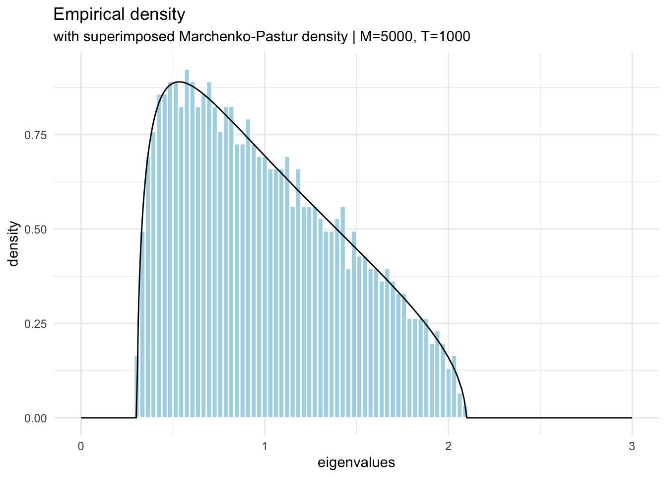
Random correlation matrices

We have $M$ variables with $T$ rows. The elements of the $M\times M$ empirical correlation matrix $E$ are given by:

$$E_{i,j}=\frac{1}{T}\sum_{t=1}^Tx_{i,j}x_{j,i}$$ where $x_{i,j}$ denotes the $j$-th (normalized) value of variable $i$. This can be written as $E=H^\top H$ where $H$ is the $T\times M$ dataset.

Assuming the values of $H$ are random with variance $\sigma^2$ then in the limit $T,M\rightarrow\infty$, while keeping the ratio $Q\equiv\frac{T}{M}\ge1$ constant, the density of eigenvalues of $E$ is given by

$$\rho\left(\lambda\right) = \frac{Q}{2\pi\sigma^2}\frac{\sqrt{\left(\lambda_+-\lambda\right)\left(\lambda-\lambda_-\right)}}{\lambda}$$ where the minimum and maximum eigenvalues are given by

$$\lambda_\pm=\sigma^2\left(1\pm\sqrt{\frac{1}{Q}}\right)^2$$

is also known as the Marchenko-Pastur distribution that describes the asymptotic behavior of eigenvalues of large random correlation matrices.

mpd <- function(lambda,T,M,sigma=1){
  Q <- T/M
  lambda_plus  <- (1+sqrt(1/Q))^2 * sigma^2
  lambda_minus <- (1-sqrt(1/Q))^2 * sigma^2
  if(lambda < lambda_minus | lambda > lambda_plus){
    0
  }else{
    (Q/(2*pi*sigma^2)) * sqrt((lambda_plus-lambda)*(lambda-lambda_minus)) / lambda
  }
}

M = 1000, T = 5000

t <- 5000;
m <- 1000;
h = array(rnorm(m*t),c(m,t)); # Time series in rows
e = h %*% t(h)/t; # Form the correlation matrix
lambdae = eigen(e, symmetric=TRUE, only.values = TRUE);

# create the mp distribution
mpd_tbl <- tibble::tibble(lambda = c(lambdae$values, seq(0,3,0.1)) ) |> 
  dplyr::mutate(mp_dist = purrr::map_dbl(lambda, ~mpd(lambda = ., t,m)))

# plot the eigenvalues
tibble::tibble(lambda = lambdae$values) |> 
  dplyr::mutate(mp_dist = purrr::map_dbl(lambda, ~mpd(lambda = ., t,m))) |> 
  ggplot(aes(x = lambda, y = after_stat(density))) + 
  geom_histogram(color = "white", fill="lightblue", bins=100) + 
  geom_line(data = mpd_tbl, aes(y=mp_dist)) +
  labs(x = 'eigenvalues', title = 'Empirical density'
  , subtitle = 
    stringr::str_glue("with superimposed Marchenko-Pastur density | M={t}, T={m}")
  ) +
  xlim(0,3) +
  theme_minimal()

M = 100, T = 500

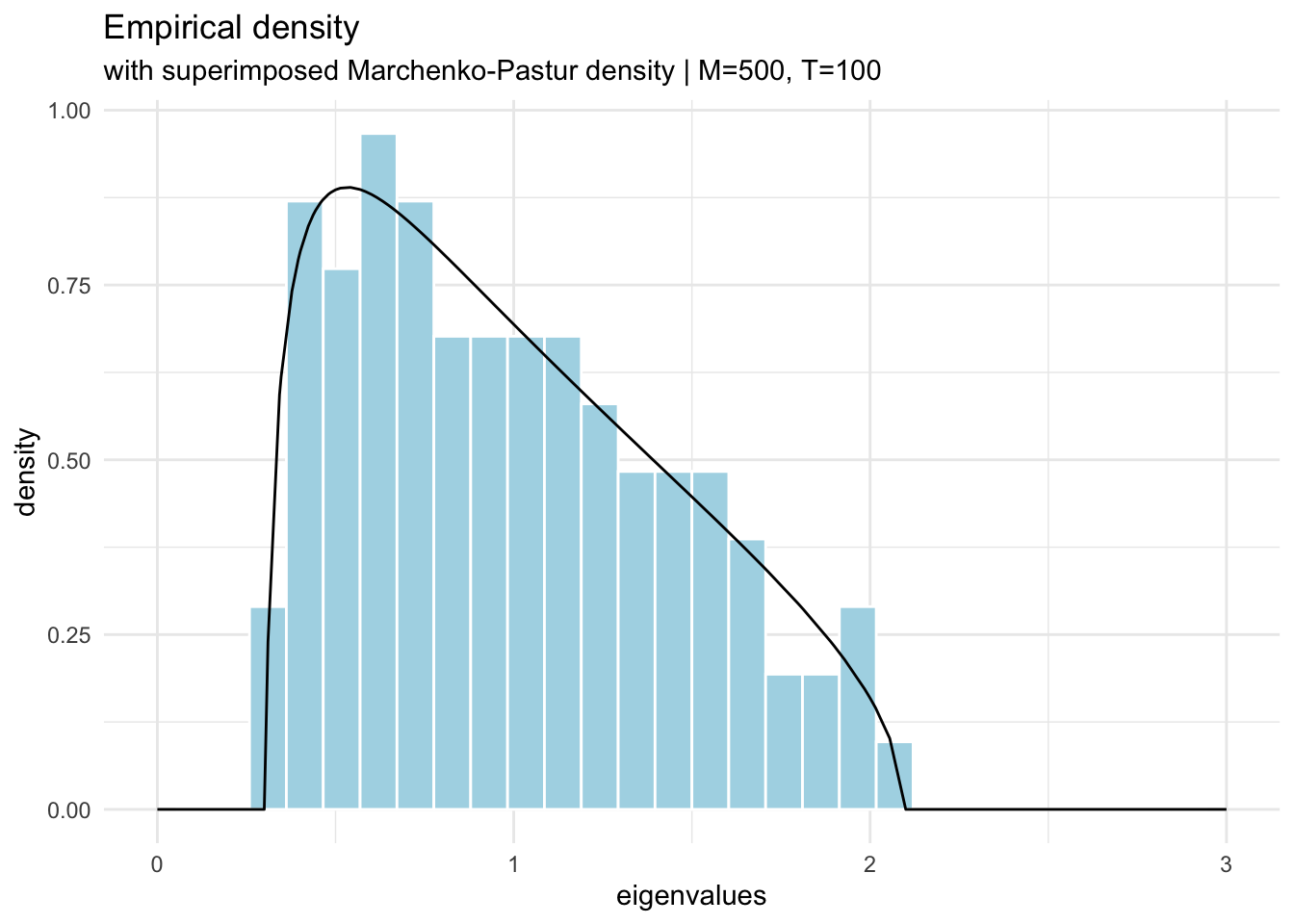
t <- 500;
m <- 100;
h = array(rnorm(m*t),c(m,t)); # Time series in rows
e = h %*% t(h)/t; # Form the correlation matrix
lambdae = eigen(e, symmetric=T, only.values = T);

# create the mp distribution
mpd_tbl <- tibble::tibble(lambda = c(lambdae$values, seq(0,3,0.1)) ) |> 
  dplyr::mutate(mp_dist = purrr::map_dbl(lambda, ~mpd(lambda = ., t,m)))

# plot the eigenvalues
tibble::tibble(lambda = lambdae$values) |> 
  dplyr::mutate(mp_dist = purrr::map_dbl(lambda, ~mpd(lambda = ., t,m))) |> 
  ggplot(aes(x = lambda, y = after_stat(density))) + 
  geom_histogram(color = "white", fill="lightblue", bins=30) + 
  geom_line(data = mpd_tbl, aes(y=mp_dist)) +
  labs(x = 'eigenvalues', title = 'Empirical density'
  , subtitle = 
    stringr::str_glue("with superimposed Marchenko-Pastur density | M={t}, T={m}")
  ) +
  xlim(0,3) +
  theme_minimal()

M = 10, T = 50

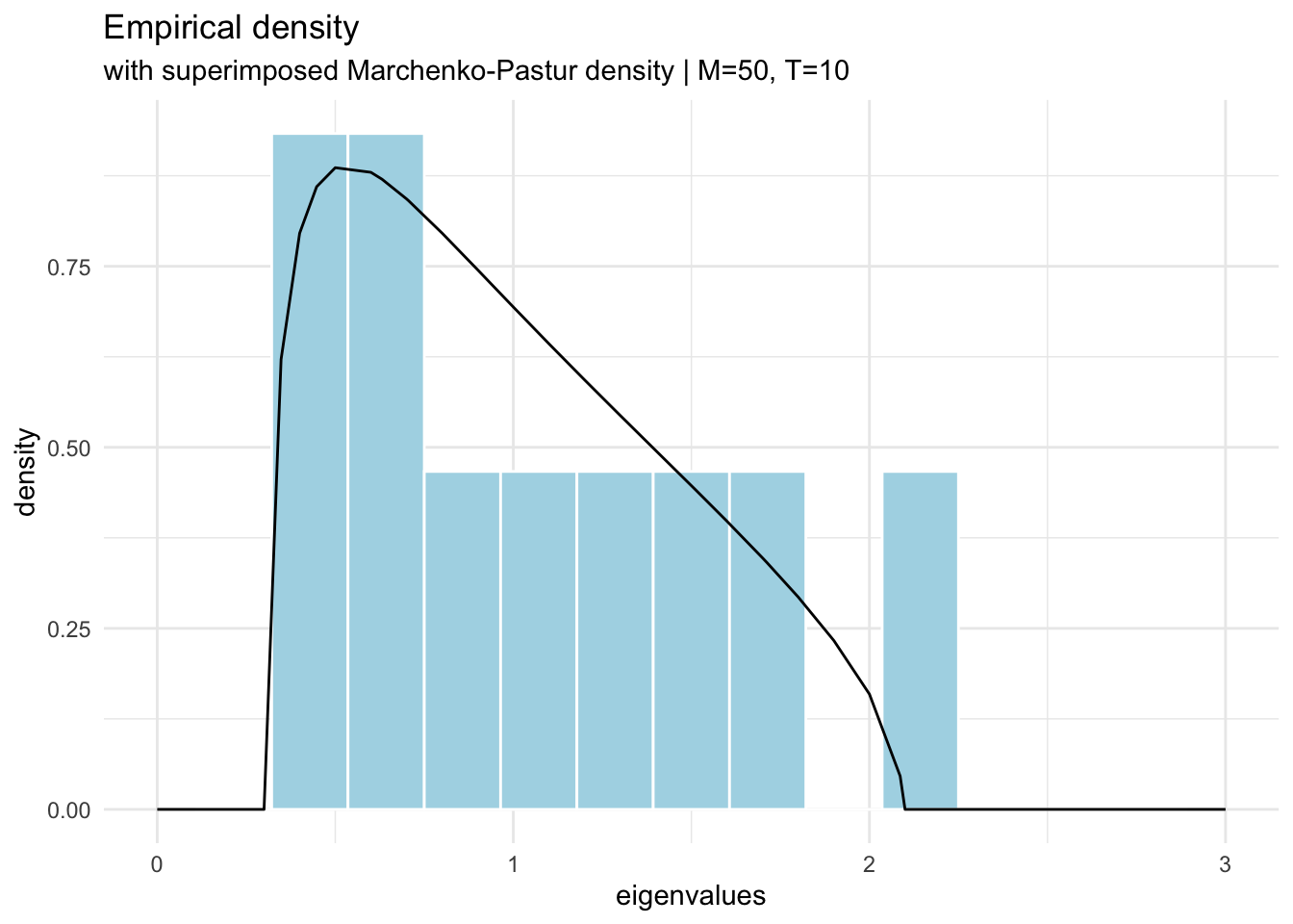
t <- 50;
m <- 10;
h = array(rnorm(m*t),c(m,t)); # Time series in rows
e = h %*% t(h)/t; # Form the correlation matrix
lambdae = eigen(e, symmetric=T, only.values = T);

# create the mp distribution
mpd_tbl <- tibble::tibble(lambda = c(lambdae$values, seq(0,3,0.1)) ) |> 
  dplyr::mutate(mp_dist = purrr::map_dbl(lambda, ~mpd(lambda = ., t,m)))

# plot the eigenvalues
tibble::tibble(lambda = lambdae$values) |> 
  dplyr::mutate(mp_dist = purrr::map_dbl(lambda, ~mpd(lambda = ., t,m))) |> 
  ggplot(aes(x = lambda, y = after_stat(density))) + 
  geom_histogram(color = "white", fill="lightblue", bins=15) + 
  geom_line(data = mpd_tbl, aes(y=mp_dist)) +
  labs(x = 'eigenvalues', title = 'Empirical density'
  , subtitle = 
    stringr::str_glue("with superimposed Marchenko-Pastur density | M={t}, T={m}")
  ) +
  xlim(0,3) +
  theme_minimal()

Application to correlation matrices

For the special case of correlation matrices (e.g. PCA), we know that $\sigma^2=1$ and $Q = T/M$. This bounds the probability mass over the interval defined by $\left(1\pm\sqrt{\frac{1}{Q}}\right)^2$.

Since this distribution describes the spectrum of random matrices with mean 0, the eigenvalues of correlation matrices (read PCA component weights) that fall inside of the aforementioned interval could be considered spurious or noise. For instance, obtaining a correlation matrix of 10 variables with 252 observations would render

$$\lambda_+=\left(1\pm\sqrt{\frac{1}{Q}}\right)^2\approx1.43$$

Thus, out of 10 eigenvalues/components of said correlation matrix, only the values higher than 1.43 would be considered significantly different from random.